Wednesday, April 27, 2016

Selected Twitter Quotes


Monday, April 25, 2016

The Problem with Facebook and Global Variables

A few years ago, Facebook was a source of joy in my life. I was actively rediscovering friends who had slipped away over time. Reconnecting, discovering what they were up to, and filling the gap between where we had left and found each other again, ushered in a sense of everyday freshness.

Over time, as a billion people got onboard, the rate of rediscovery diminished, and so did the excitement of eagerly checking new notifications. These days, most of my Newsfeed is cluttered with click-bait, unscientific bullshit, flashy headlines, and "Hallmark" greetings.

Every now and then, somebody posts pictures of an event or vacation, or something extraordinarily interesting. Those mark the high points; the rest is mostly junk.

I don't have the Facebook app on my phone. I've pretty much stopped contributing anything original myself like so many others. The other day I was thinking about why I stopped posting, and it occurred to me that my "friends" list contains contains a motley group of people who I know in very different ways.

We are different to different people. We are different to our kids, to our parents, our friends from undergrad, our professional colleagues, our bosses etc. This is not hypocrisy. This is human nature.

Trying to post something that does not offend at least one of the groups I belong to is either uninteresting or impossible.

Because of a conversation I had earlier today, I couldn't help noticing the parallels of this "context collapse", with global variables in programming. While useful as a hack, when the program (friend network) is small, global variable ("global" posts) seriously screw things up, as the program begins to scale.

If you post something, or declare a global variable, everyone and everything can see it. When you have 20 friends, or a 20-line program, this is not much of a problem. You can use your sense of smell to detect problems, and fix them as needed.

But these beasts, they live on forever. They cause unforeseen errors and gaffes.

In the programming world, the solution is encapsulation; defining variables within a context or a subroutine. These variables are invisible to the rest of the program. They arise as soon as control flows in, and die as control flows out.

For large software projects, this is not just a good idea, but a necessary idea. You shouldn't have to worry about the entire universe getting screwed up, just because you changed the name of a variable.

To be fair, Google+ and Facebook do allow you to customize and limit the scope of pictures and comments you post. That is, encapsulation is possible. But it is cumbersome, and I don't know many people who use it skillfully. Programming is work; posting on Facebook is supposed to be fun.

This probably explains the rising popularity of messaging apps (iMessage, WhatsApp, Snapchat) where group identity is a fundamental building block. Groups automatically provide localized contexts. The proportion of original content that people feel comfortable posting on messaging apps is so much higher.

Thursday, April 21, 2016

Thoughts on Truncation and Round-off Errors

In scientific computing or numerical analysis, truncation and roundoff errors pop up all over the place. In some operations the former dominates, in others it is the latter, and in a few others, they both conspire in surprising ways.

Truncation error is "is the error made by truncating an infinite sum and approximating it by a finite sum". Or as I sometimes like to say, "somewhere a Taylor series is truncated, and it is not happy!" 

For example, in numerical quadrature, different Newton-Cotes formulas may be derived by locally "fitting" the integrand function with polynomial approximations (Taylor series), and computing the area under the polynomial, since it is much easier to do.

In the solution of ordinary differential equations using Runge-Kutta or linear multistep methods, one tries to perform a term-by-term comparison with a Taylor series expansion, and use polynomial interpolation of the recent past, respectively, to develop different formulas.

In these operations, from a practical standpoint, truncation error dominates!

Roundoff error is the difference between a mathematical number and its finite precision computer representation. It is purely an artifact of the fixed word size used in modern computers. It often dominates the conversation, when subtraction of nearly equal numbers is carried out numerically.

For instance, in solving a system of linear equations, the idea is to take linear combinations of equations to subtract and zero out certain coefficients. In linear systems, there is clearly no Taylor series, and roundoff error is the root cause of ill-conditioning. In fact, if we had infinitely precise number representation on computers, it might be argued that we don't have to worry about conditioning at all!

Since linear systems are at the root of nearly all problems in scientific computing, round-off error is always lurking around the corner.

There are some spectacular cases like numerical differentiation where both roundoff error and truncation error play an "equally" important role. In deriving finite difference formulae, we truncate appropriate Taylor expansions. Furthermore, the derivative itself involves ratios of differences of nearly identical terms.

Monday, April 18, 2016

What I Learned Last Week

1. You cannot speed read (NYT)
Our favorite Woody Allen joke is the one about taking a speed-reading course. “I read ‘War and Peace’ in 20 minutes,” he says. “It’s about Russia.” 
... the big bottleneck in reading isn’t perception (seeing the words) but language processing (assembling strings of words into meanings).
 2. The power of salt water (via @MaxVenerator)
"The cure for anything is salt water: sweat, tears, or the ocean." ~ Isak Dinesen
3. David MacKay passed away (The Telegraph) : His book on alternative energy (without the hot air), with a focus on common sense and basic numeracy, shaped a lot of my current thinking on energy and the human race, about 6 years ago.

4. The Motorway or Steiner Problem


5. Concept Creep and Safe Spaces on College Campuses (The Guardian)

Saturday, April 16, 2016

What is Computational Science?

I have been in the Department of Scientific Computing at Florida State University for close to a decade now. Since computational science or scientific computing is a relatively new "department", I often have to explain, what it is exactly that we, computational scientists do.

My usual answer runs something like this: computational science is a relatively new discipline that sits at the intersection of computer science, mathematics, and science and engineering.

Traditionally, computer science deals with the design and analysis of data-structures, operating systems, compilers, networks, computer architectures and algorithms.

Similarly, mathematics, especially applied math, deals with application of math to science and engineering. Folks in applied math like to prove theorems about the existence and uniqueness of solutions, and the convergence of numerical schemes. Sometimes, they might not even need computers, and even when they do, they might not necessarily need big computers.

Science and engineering might include various traditional disciplines such as geology, mechanical engineering, biology, materials science, physics, etc. People in traditional science and engineering departments use a combination of theory, experiments, and models. Some of these models may be complicated enough to require computers.

Loosely, we may describe computational scientists as people who, develop algorithms that use computers to advance science.

While there is a lot of diversity among computational scientists, a typical workflow may look like:

  1. Develop a mathematical model of a science or engineering problem. For example, this may be a continuous partial differential equation description of fluid flow.
  2. Express it in a form suitable for computers to understand. This may involve discretizing the domain into a mesh, and rewriting the differential equations as a set of discrete linear or non-linear equations.
  3. Build algorithms that are fast, and accurate to solve the systems of equations
  4. Assemble computer software by integrating available libraries with new code
  5. Analyze and visualize results. Use them to predict or to gain insights.
  6. If needed iterate. Go back to step 1, and improve the model, the discretization, the algorithm, or the computer code.

Thursday, April 14, 2016

On Middlemen

I recently heard a very interesting podcast on EconTalk on the crucial role that middlemen play in the functioning of a modern economy. It made me want to go back and hear a related podcast with Mike Munger.

Marina Krakovsky, who was the guest on the recent episode, summarized some of her positions in her blog "In Defense of the Middleman".
One of the middlemen I interviewed, the micro-VC Mike Maples, Jr., put it well when he pointed out that in our highly connected world, “things and entities that accelerate connections are going to be more valuable.” This is why Maples is bullish on so many Internet businesses, having made early investments in Twitter, Lyft, and TaskRabbit, among others. “That’s what a middleman does,” Maples says: “They connect nodes in a network to increase the value of the network.
The six primary roles of a middleman listed towards the end of the blog, and the numerous examples made me ponder for quite a while one why middlemen are so despised, when they provide such an important service.

Sorry, I am still pondering :).

Tuesday, April 12, 2016

Ralston's Method Controversy

Earlier this semester, I was teaching second-order Runge-Kutta methods, when one of my students, Eitan Lees, noticed that the formulas I wrote down for Ralston's method, was inconsistent with the formula on wikipedia and elsewhere on the web. This form can be written in the famous "RK Tableau" form as: \[\begin{array}{c|cc}
0   & 0   & 0  \\
2/3 & 2/3 & 0  \\
\hline
    & 1/4   & 3/4  \\
\end{array}.\] However, there are other sources on the web, and the famous textbook of Chapra and Canale, which give a different formula (and the one I happened to use in my class, probably because I picked it up from that very source). This has the form: \[\begin{array}{c|cc}
0   & 0   & 0  \\3/4 & 3/4 & 0  \\
\hline
    & 1/3   & 2/3  \\
\end{array}.\] Ralston's method is special, because it promises to be the "best" explicit RK2 method. What is more, I distinctly remember seeing an example in the C&C textbook pitting their version of the method against the competition (other explicit RK2 methods) and showing that it was indeed the best!

So which of the two forms is correct. There can't really be two best RK2 methods, can there?

I looked at the original source, the 1962 paper by Ralston, and the book "A First Course in Numerical Analysis" by Ralston, and found that the original versions favor the wikipedia form.

From Ralston, 1962; more on this later.
Surprisingly, Chapra and Canale cite these two sources before they put down their (what turns out to be incorrect) form.

Background on Explicit RK2 

To back up a little bit, the family of second order RK methods are given by,\[y_n = y_{n-1} + h (a_1 k_1 + a_2 k_2),\] where, \[\begin{eqnarray}
k_1 & = & f(t_{n-1}, y_{n-1}) \\
k_2 & = & f(t_{n-1} + p_2 h , y_{n-1} + q_{21} k_1 h)
\end{eqnarray}.\] Using Taylor series expansion, and linearizing \(k_2\) it can be shown that coefficients have to satisfy the constraints, \[\begin{align*}
  a_1 + a_2 & = 1 \\
  a_2 p_2 & = \frac{1}{2} \\
  a_2 q_{21} & = \frac{1}{2}
\end{align*}.\] If one of the four unknowns is specified (say \(a_2\)) the other unknowns can be determined easily.

So there is a family of RK2 methods.
  • Heun's Method: \[a_2 = 1/2; \implies a_1 = 1/2,~ p_2 = q_{21} = 1.\]
  • Midpoint Method: \[a_2 = 1; \implies a_1 = 0, p_2 = q_{21} = 1/2.\]
  • Ralston's Method (1 - 1962 paper): \[a_2 = 3/4; \implies a_1 = 1/4, p_2 = q_{21} = 2/3.\]
  • Ralston's Method (2 - C&C text):  \[a_2 = 2/3; \implies a_1 = 1/3, p_2 = q_{21} = 3/4.\]
Error Analysis 

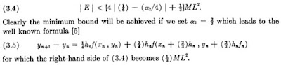
One can follow Ralston's analysis in his 1962 paper. In the paper he shows that his method can be obtained by trying to minimize a bounding function
\[|E| < \left(4 \left| \frac{1}{6} - \dfrac{p_2}{4} \right| + \dfrac{1}{3} \right)ML^2,\] I have rewritten this portion (which can be seen from the picture excerpted from the original paper above) in my notation. Note that \(p_2\) in our case is the same as \(\alpha_2\) in the 1962 paper.

It is easy to see that the minimum is obtained at \(p_2 = 2/3\). In fact, one can plot this error bound function, and locate the different RK2 methods on it.


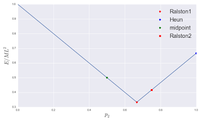
One can see the location of the actual optimum (2/3), the Ralston's method reported in Chapra and Canale (red square = Ralston2), and the other two RK2 methods.

In terms of error bound, one notes that ordering the method from most to least accurate, we have:

  • Ralston 1 (1962 form)
  • Ralston 2 (C&C text)
  • Midpoint Method
  • Heun's Method

Test Example

Chapra and Canale do a numerical example in which their version of Ralston's method (Ralston2) outperformed both Heun's and midpoint method. \[y'(t) = -2 t^3 + 12 t^2 - 20t + 8.5,~~~y(0) = 1.\] This is an interesting example because the RHS is only a function of \(t\), and this is in fact a quadrature problem masquerading as an initial value problem.


It is simple enough that one can easily find the exact analytical solution, and hence compute the true error in a numerical method. All RK2 methods are second order accurate (\(\mathcal{O}(h^2)\)), where h is the step-size.

Here is how the 4 different RK2 methods perform:


As you see, the order of accuracy of Heun's method, midpoint method, and the C&C version of Ralston method is as expected from the error analysis. The dashed line has a slope of 2, and shows that the three methods are second ordered.

The true Ralston method (Ralston1) is an outlier and is far more accurate than the other three. Curiously, it also has a higher slope. The slope of the dotted line is 3. What happened was that the choice of \(p_2\) reduced the constant in front of the \(\mathcal{O}(h^2)\) term to such an extent that it neutralized that term, and conspired to give us an serendipitous boost of one order in accuracy. The dotted line has a slope of 3.

Conclusion

A possible origin of this discrepancy is that Ralston called \(p_2\) as \(\alpha_2\) in his original paper. It is possible that the \(\alpha_2 = 2/3\) got confused with \(a_2 = 2/3\) in the C&C textbook. Given the popularity of the textbook, the mistake proliferated inadvertently.

This is why you need smart students constantly questioning received wisdom.

Friday, April 8, 2016

Extracting Data from Static Plots

In the past, I have used two programs to extract datapoints from a graph. The typical use case is to save the coordinates extracted from a pdf or png graph, so that you can use them for calculations or to overlay on your graphs.

1. DataThief: A shareware program that is cross platform. It is written in Java and works on Windows, MacOS, and Linux.

2. Engauge Digitizer: This is also cross platform. I have written a little bit about using it here.

In the past month, I discovered WebPlotDigitizer.

It is completely web-based, so on doesn't have to "install" it. This means, it is completely blind to the underlying operating system. The interface overall seems much spiffier, but I haven't taken it out for a serious test drive.

Saturday, April 2, 2016

Jupyter Tricks

I recently learned a useful trick: use %matplotlib notebook instead of %matplotlib inline for interactive plots.

That led me to look for more Jupyter tricks, and I found two useful sites